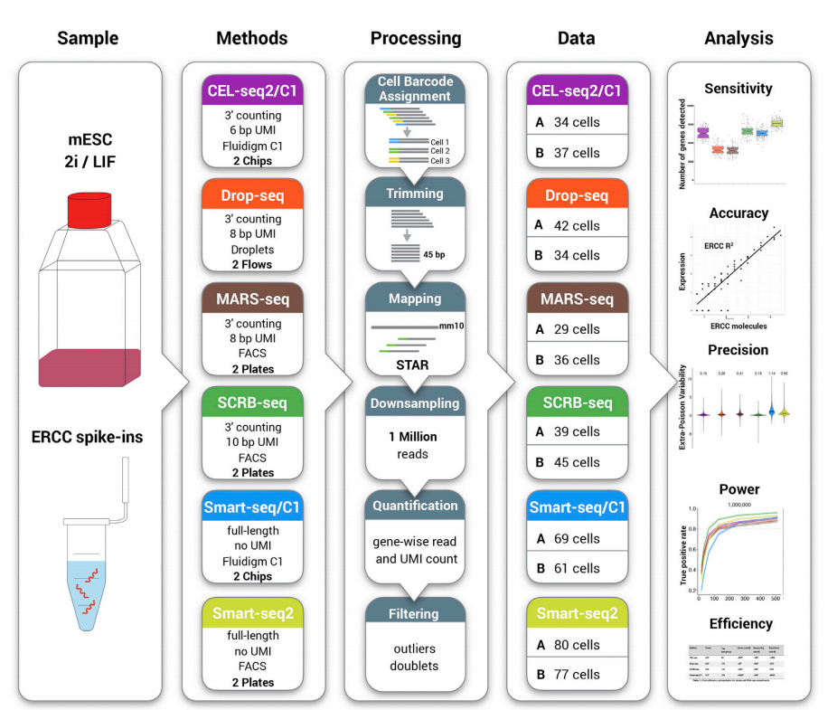
Smart-seq2是一种单细胞RNA测序技术,用于分析单个细胞的基因表达情况,并可以对单个细胞的基因表达进行分析。
通过设计oliGo(dT)VN Primer作为逆转录引物,利用MMLVRT的模板转换活性,在cDNA的3’端添加一段接头序列,通过该接头序列进行反转录,生成cDNA第一条链。当逆转录酶到达mRNA5’末端时,会连续在末端添加几个胞嘧啶(C)残基。然后添加TSO(template-switching oliGo)引物,退火后结合在第一条链的3’端与poly(C)突出杂交,合成第二条链。这样得到的cDNA经过PCR扩增,然后再纯化后用于测序。
| Pipeline Features | Description | Source |
|---|---|---|
| Assay Type | paired-end plate-based Smart-seq2 | |
| Overall workflow | Quality control module and transcriptome quantification module | Code available from Github |
| Workflow language | WDL | openWDL |
| Genomic reference sequence | GRCh38 human genome primary sequence | GENCODE |
| Gene Model | GENCODE v27 PRI GTF and Fasta files | GENCODE |
| Aligner | HISAT2 | Kim, et al.,2015; HISAT2 tool |
| QC | Metrics determined using Picard command line tools | Picard Tools |
| Estimation of gene Expression | RSEM (rsem-calculate-expression) is used to estimate the gene expression profile. The input of RSEM is a bam file aligned by HISAT2. | Li and Dewey, 2011 |
| Data Input File Format | File format in which sequencing data is provided | FASTQ |
| Data Output File Format | File formats in which Smart-seq2 pipeline output is provided | BAM, Zarr version 2 |
首先,需要对原始测序数据进行质控和比对。质控可以使用FastQC和MultiQC工具来检查数据质量。比对可以使用HISAT2工具,将测序数据比对到参考基因组1。
# 质控 fastqc -t 6 -o ./fastqc_result ./RAW/SRR*fastq.gz multiqc ./fastqc_result使用featureCounts工具对比对后的BAM文件进行定量,生成基因表达矩阵2。
featureCounts -T 10 -p -t exon -g gene_name -a annotation.gtf -o counts.txt *.bam 基本批量运行流程如下:#!/bin/bash
# 检查是否安装了GNU Parallel
if ! command -v parallel &> /dev/null; then
echo "GNU Parallel could not be found, please install it first."
exit 1
fi
# 创建namelist文件,列出所有样本文件夹名称
ls -d */ > namelist
# 定义进一步处理RNA序列的函数
process_rna() {
local sample=$1
# 去除末尾的斜杠
sample=$(echo "$sample" | sed 's:/*$::')
echo "${sample} RNA processing start"
if [ ! -d "${sample}" ]; then
echo "Directory ${sample}does not exist, skipping."
return
fi
cd "${sample}" || { echo "Failed to enter ${sample}"; continue; }
source /data5/xxx/zengchuanj/Software/MACS3/MyPythonEnv/bin/activate
trim_galore -j 20 --phred33 --gzip --trim-n -o result --paired *.fastq.gz
cd result
source /data5/tan/zengchuanj/conda/bin/activate
conda activate HiC-Pro
fastp -i "../${sample}_clean_R1.fastq.gz" -I "../${sample}_clean_R2.fastq.gz" -o "${sample}_clean_R1.fq.gz" -O "${sample}_clean_R2.fq.gz" -q 20 -w 16 -n 5
fastqc -t 10 "${sample}_clean_R1.fq.gz" "${sample}_clean_R2.fq.gz"
hisat2 -p 20 -x /data5/tan/zengchuanj/pipeline/HIC/juicer/references/mm10/mm10 -1 ${sample}_clean_R1_val_1.fq.gz -2 ${sample}_clean_R2_val_2.fq.gz 2>"${sample}_hisat.txt" | samtools view -o "${sample}_outname.bam"
samtools sort -@ 20 -o ${sample}.sort.bam ${sample}_outname.bam
##featurecounts定量
# 使用ensamble的GTF
echo ${sample} 'Feature counts start'
### (ucsc的话 -t exon)
# 根据gene与exon调整参数
featureCounts -p --countReadPairs -T 20 -t gene -a /data5/xxx/zengchuanj/xxx/references/GTF/Mus_musculus.GRCm38.102.gtf -o ${sample}_count.txt ${sample}.sort.bam
echo "${sample} RNA processing finish"
cd ../../..
}
# 使用parallel并行处理每个样本,并限制最大线程数为15
export -f process_rna
# 并行进一步处理RNA序列
parallel -j 10 process_rna ::: $(cat namelist)# 定义一个用于处理Smart-seq数据并创建Seurat对象的函数
process_smart_to_seurat_data <- function(file_path,project = "seurat_obj") {
gc()
library(clusterProfiler)
library(org.Mm.eg.db)
library(Seurat)
# 读取数据
result <- read.csv(file_path,header = T,check.names = FALSE)
print(head(result))
# 设置行名并移除gene列
rownames(result) <- result$gene
result <- result[,-1]
# 转换基因ID
hg <- bitr(result$gene, fromType="ENSEMBL", toType=c("ENTREZID","ENSEMBL","SYMBOL"), OrgDb="org.Mm.eg.db")
num <- match(hg$ENSEMBL, result$gene)
result$gene[num] <- hg$SYMBOL
# 移除重复项并重组数据
un <- unique(result$gene)
ma <- match(un, result$gene)
data <- result[ma, ]
rownames(data) <- data$gene
data <- data[,-1]
print(head(data))
# 用0填充
data[is.na(data)] <- 0
# 创建Seurat对象
seurat_obj <- CreateSeuratObject(counts = data, project = project)
return(seurat_obj)
}
# 仅仅只转换gene名
process_smartseq_data <- function(file_path) {
gc()
library(clusterProfiler)
library(org.Mm.eg.db)
library(Seurat)
# 读取数据
result <- read.csv(file_path,header = T,check.names = FALSE)
print(head(result))
# 设置行名并移除gene列
rownames(result) <- result$gene
result <- result[,-1]
# 转换基因ID
hg <- bitr(result$gene, fromType="ENSEMBL", toType=c("ENTREZID","ENSEMBL","SYMBOL"), OrgDb="org.Mm.eg.db")
num <- match(hg$ENSEMBL, result$gene)
result$gene[num] <- hg$SYMBOL
# 移除重复项并重组数据
un <- unique(result$gene)
ma <- match(un, result$gene)
data <- result[ma, ]
rownames(data) <- data$gene
data <- data[,-1]
print(head(data))
# 用0填充
data[is.na(data)] <- 0
return(data)
}在进行下游分析之前,需要对数据进行标准化和过滤。可以使用Seurat包进行数据标准化和高变基因筛选1。
library(Seurat)
sce <- CreateSeuratObject(counts = counts_matrix, project = "sce_project", min.cells = 1, min.features = 0)
sce <- NormalizeData(sce)
sce <- FindVariableFeatures(sce, selection.method = "vst", nfeatures = 2000)
使用PCA和tSNE进行数据降维,并使用Seurat包进行聚类分析1。
sce <- ScaleData(sce, vars.to.regress = c('nUMI_raw'))
sce <- RunPCA(sce, features = VariableFeatures(object = sce))
sce <- FindNeighbors(sce, dims = 1:20)
sce <- FindClusters(sce, resolution = 0.3)
sce <- RunTSNE(sce, dims = 1:9)
DimPlot(sce, reduction = "tsne")
使用monocle包进行差异基因分析,识别不同细胞群体之间的差异基因1。
library(monocle)
DE_sce <- prepare_for_DE(count_matrix, clustering, stages)
DE_genes <- findDEgenes(DE_sce, qvalue = 0.05)
对差异基因进行功能注释,使用clusterProfiler包进行GO富集分析3。
library(clusterProfiler)
entrez_genes <- bitr(de_genes$genes, fromType = "SYMBOL", toType = "ENTREZID", OrgDb = "org.Mm.eg.db")
formula_res <- compareCluster(ENTREZID ~ cluster, data = de_gene_clusters, fun = "enrichGO", OrgDb = "org.Mm.eg.db", ont = "BP", pAdjustMethod = "BH", pvalueCutoff = 0.01, qvalueCutoff = 0.05)
dotplot(formula_res, showCategory = 5)